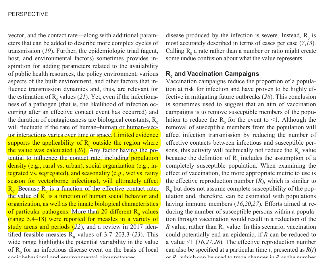
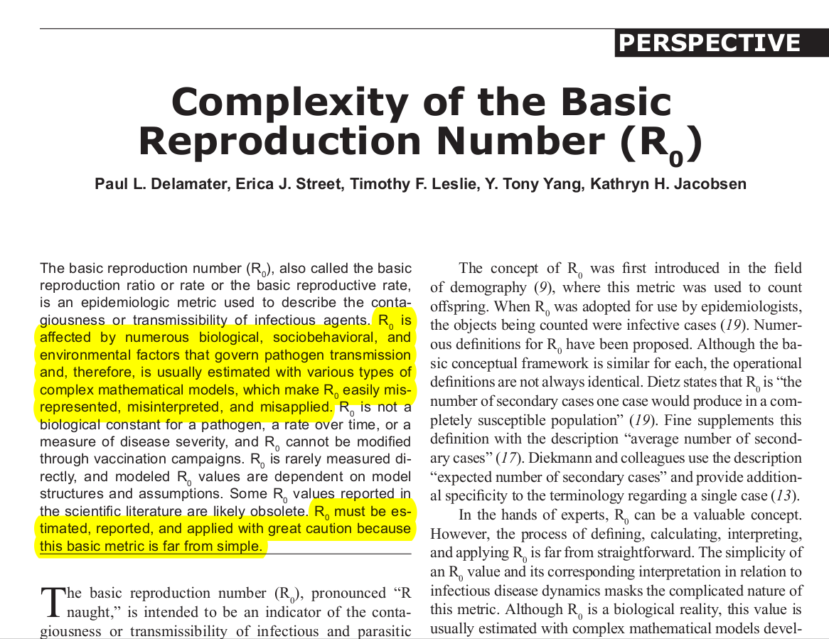
Currently accepted views on contagion are based on the concept of Transmission Chains (aka Chains of Infection) [1] and are usually described by very simplified and reductionist Compartmental Models in Epidemiology [2] such as the SIR model (Susceptible-Infectious-Recovered); which are characterized by the Basic Reproduction Number (R_0). However the complexity of R_0 is very often misrepresent as a constant capable of characterizing the transmissibility of infectious agents, when in reality it is a function that must be estimated via mathematical modelling under different assumptions and cannot be readily applied outside of the region where it was calculated [3].

In a previous article [4] we already defined the complexity of such function, in terms of a potential landscape Φ (the contagion landscape, CL), as follows:
R_0(Φ)=> CL = Φ[Ψ_1( Ψ_2(), Ψ_3(), ... , Ψ_n(), Time, Physical Constants, Biological Constants, Local Constants, Constants Dependent on Time (C(t)) ); Ψ_2( Ψ_1(), Ψ_3(), ... , Ψ_n(), Time, Physical Constants, Biological Constants, Local Constants, C(t)); ... ; Ψ_n( Ψ_1(), Ψ_2(), ... , Ψ_(n-1)(), Time, Physical Constants, Biological Constants, Local Constants, C(t)); Time, Physical Constants, Biological Constants, Local Constants, C(t)); ]
where the primary variables (Ψ_1(), Ψ_2(), ... , Ψ_n()), which are variables of each other and time, and some of the constants, are:
(age, gender, previous comorbidities, previous general health, environmental toxins, contaminants, pharmacological products usage, nutrition levels, living conditions, livelihood, poverty levels, hygiene, climate/weather, latitude, geography, local flora, local fauna, air quality, water quality, food quality, immunological memory/strength - at the ecosystemic level and at the individual level -, culture, behavior, genetic variation, population density, location within the urban environment, dynamics, temporal variations, humidity, solar radiation, temperatures, electromagnetic fields, fitness levels, time of the year, time of the day/week, ad infinitum...)
Thus, as the reader can appreciate, the complexity of this apparently straightforward and trivial parameter (R_0) is considerably high. In fact, a new model of contagion is required to properly understand the meaning of it. From previous work [5]:
“It is not the presence of molecular patterns (e.g. viruses, bacteria, fungi…) what moves from individual to individual causing disease. For the most part, such elements are ubiquitous throughout the ecosystem, that is, they are already present; and the relevant biological pathways related to them behave as if they were in a state of equilibrium or quasi-equilibrium, state in which they are harmless or even beneficial and needed for the proper function of the associated biological functions of the whole ecosystem. What moves are waves of non-equilibrium states.”
If we take this new approach in relation to infectious diseases, non-equilibrium states and the probability flux between different attractors within the contagion landscape, constitute the most relevant factors that we should take into consideration. Such perspective can be described by Potential Landscape & Flux Theory of Non-Equilibrium Dynamical Systems. Plenty of research has been done in this direction in an attempt to better describe biological systems [6,7,8], such as protein folding, evolution, ecology, the cell cycle and cell differentiation, cancer, neural networks...
We still need to remember that assumptions are required in order to characterize the dynamics of the system under study, which could lead to considerably misleading results if important drivers or attractor states are not considered or very broad simplifications are applied, as it tends to be the case in epidemiological models of disease (e.g. the SIR model).
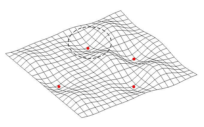
Let’s consider now a very simple attractor landscape (image from [9]) to illustrate what a contagion landscape might actually look like.

As we can see, in this example there are four main attractors, which could describe the following states:
1. Healthy with True Negative results for infectious agent A.
2. Healthy with True Positive results for infectious agent A.
3. Unhealthy with Clinical Symptoms for disease A & True Negative results for infectious agent A.
4. Unhealthy with Clinical Symptoms for disease A & True Positive results for infectious agent A.
As we said earlier, this particular contagion landscape belongs to a given area/location and a given point in time. If we were to study an epidemic situation in such location with a given population of size N, the estimated R_0 for disease A would only apply to that particular location and point in time. Fluctuations of its value and the dynamical behavior would not be captured. However statistics derived from such estimate would be carelessly apply to SIR models, public health policies and intervention strategies, while its descriptive value is extremely narrow and constraint, making such interventions probably more harmful than beneficial.
If we were to consider the contagion landscape as a whole instead, we would be able to properly characterize the actual dynamics of the disease in terms of non-equilibrium states rather than the presence or absence of a given molecular pattern within the population. It would be very easy to notice, paying attention to ecosystemic conditions and other environmental cues, that the presence or absence of the given infectious agent is very rarely the causative/etiological factor **(see note below for the definition of etiological factor in this context). Proliferation of the agent into a disease state would require a particular set of conditions (described above within the primary variables of the contagion landscape). Example:
Scenario 1) Let’s imagine that the given landscape is divided into 2 regions with a population of N/2 each. In region 1 humidity is high, ventilation is low and the concentration of a given species of mold in the air is above a given threshold. In region 2 the conditions are the same however the concentration of mold is below a given threshold. Now let’s imagine that in both regions infectious agent A is present with equal number of true positive tests, however only in region 1 clinical symptoms from disease A are observed.
+ By paying attention only to the number of true positives for infectious agent A, one would obtain contradictory results. If we also pay attention to environmental cues but mold is not considered, we still have inconclusive results. Only by considering the whole contagion landscape, which includes unknown variables, one might start to investigate the true etiological factor, which in this case is the presence of mold. Infectious agent A might or might not be require to be present for the disease to take hold in the community, in this case. Farther analysis would be required.
Scenario 2) The conditions are the same as in scenario 1, however in region 2 humidity is low and ventilation is high.
+ In this case, we would, most likely, arrive (if environmental cues are considered) to the conclusion that the causative agent is the combination of humidity and ventilation, in addition to the infectious agent. However, this conclusion would be incorrect. Thus, to revisit current assumptions is always a requirement, because unknown variables will always be present. Therefore, one size fits all solutions CANNOT be readily applied.
It would be very important to pay attention to a high number of individuals within attractor 3 in this particular example. That is, ‘Unhealthy with Clinical Symptoms for disease A & True Negative results for infectious agent A’. This would indicate that infectious agent A is only correlated with disease A in some instances, however it is not directly involved in the disease course itself. Blindly applying molecular tests to any epidemic scenario would make impossible to differentiate this case.
I hope the reader can build several different scenarios where chains of infection seem to adequately describe an epidemic, regardless of whether it actually describes the true etiological factor behind it or not.
**NOTE: For clarification, the term etiological factor is used here to describe the primary factor that would eliminate the Clinical Symptoms if it is remove from the system. In the example above, removing the mold in the air would eliminate the disease state, not removing the infectious agent A. This distinction is of critical importance and very rarely taken into consideration.
References:
[1] Principles of Epidemiology _ Lesson 1 - Section 10 https://archive.cdc.gov/www_cdc_gov/csels/dsepd/ss1978/lesson1/section10.html#print
[2] Compartmental Models in Epidemiology https://pmc.ncbi.nlm.nih.gov/articles/PMC7122373/
[3] Complexity of the Basic Reproduction Number (R0) https://wwwnc.cdc.gov/eid/article/25/1/17-1901_article
[4] Our Misleading and Superstitious notion of Contagion and the Fraudulent Basic Reproduction Number in Epidemiology (+ New Perspectives) https://agustinsanchezcobos.substack.com/p/the-misleading-and-superstitious
[5] In relation to viruses as "Obligate Intracellular Parasites" and their "Pandemic" potential https://agustinsanchezcobos.substack.com/p/letter-to-dr-sam-bailey
[6] Perspectives on the landscape and flux theory for describing emergent behaviors of the biological systems https://pubmed.ncbi.nlm.nih.gov/34822073/
[7] The Potential and Flux Landscape Theory of Ecology https://journals.plos.org/plosone/article?id=10.1371/journal.pone.0086746
[8] The potential and flux landscape theory of evolution https://pubs.aip.org/aip/jcp/article-abstract/137/6/065102/72867/The-potential-and-flux-landscape-theory-of?redirectedFrom=fulltext
[9] An attractor landscape is an abstraction of the State Space of a System. It describes how the system’s Attractors are topologically distributed https://wolfgangwopperer.com/notes/attractor-landscape


In other words, epidemiology is built on a very shaky foundation defined by simple models that cannot possibly account for the extreme variability, infinite degrees of freedom, and countless unknowns present in the natural world. Hence epidemiologists cannot protect us or save us from anything. It's as if the whole field was formed to prevent us from falling off the edge of the earth.